

To start we have to set up R for generating designs. This should not be onerous in this case. The most difficult thing is in setting up the data file in the first instance (usually through a GIS). Here we have used an asc file as this is relatively easy to read into R. This file is included in the field manual package, along with the R code to create the output below.
This document was created using the R-package knitr (Xie, 2014). It is a wonderful tool, but like any tool it requires interpretation. Most notable here is that the R-code is placed in a grey box, to enable readers to highlight the code versus the document text. Within the code sections, anything that comes after a ‘#’ symbol is a comment that is not interpreted by R (most of these are a brown colour). Bold dark blue words are function names. Dark blue words are argument names. Green is for text and light blue for numbers.
###########################################################################
####    Read in Data from spatial data (.asc here) and Organise        ####
####    Foster et al. NESP Biodiversity Hub Field Manuals              ####
###########################################################################

##if you don't have MBHdesign installed, please do so using
# install.packages( "MBHdesign")

#Load required packages
library(MBHdesign) #For spatial sampling
library(fields)  #for lots of things, but for plotting in this example
library(sp)  #for reading the ascii file of cropped depths for the reserve

#Set a seed for reproducability
set.seed(666)

#Read in depth as a asc file containing long, lat and depth
#This path/file only exists on the first author's system
#   you will need to change it if running this code
#the projection will need to be changed for each region too
#bth.orig.grid <- read.asciigrid("./ExampleGovIsland/gov_bth.asc", proj4string = CRS("+proj=utm +zone=55 +datum=WGS84"))
bth.orig.grid <- read.asciigrid("gov_bth.asc", proj4string = CRS("+proj=utm +zone=55 +datum=WGS84"))

#convert to a data.frame for ease
DepthMat <- as.matrix( bth.orig.grid)
bth.orig.grid <- as.data.frame(
  cbind( coordinates( bth.orig.grid), as.numeric( DepthMat)))
colnames( bth.orig.grid) <- c("Easting", "Northing", "Depth")
bth.orig.grid <- bth.orig.grid[order( bth.orig.grid$Northing,
  bth.orig.grid$Easting),]
#Setting up plotting for now and later
uniqueEast <- unique( bth.orig.grid$Easting)
uniqueNorth <- unique( bth.orig.grid$Northing)
ELims <- range( na.exclude( bth.orig.grid)$Easting)
NLims <- range( na.exclude( bth.orig.grid)$Northing)
#Fix up ordering issue
DepthMat <- DepthMat[,rev(1:ncol(DepthMat))]
#plot it to see what we are dealing with.
image.plot( uniqueEast, uniqueNorth, DepthMat,
    xlab="Easting", ylab="Northing", main="Governor Island Reserve",
    legend.lab="Depth (m)", asp=1, ylim=NLims, xlim=ELims,
    col=rev(tim.colors()))
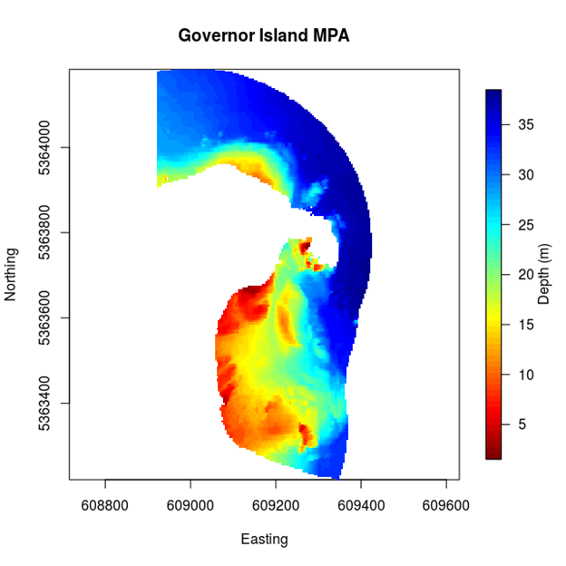
Figure 2.1: Map of Governor Island study region with depths. Note the non-regular shape and the non-uniformity of the regions depth profile.
Generate a spatially balanced design
Generating a spatially balanced design within the reserve is quite straight-forward using MBHdesign. Here we do it for 30 sampling sites spread throughout the reserve (Figure 2.1). Note that designs will vary from one realisation to the next, unless the random number generating seed is fixed (like we did in the previous subsection). Try it a few times, if you like, and see what happens between the realisations. Note that on average (over all realisations) the spatially balanced designs will have good spatial coverage.
###########################################################################
####    Spatially balanced design -- uniform inclusion probs           ####
####    Foster et al. NESP Biodiversity Hub Field Manuals              ####
###########################################################################

#number of samples
n <- 30
#take the sample
samp_spatialOnly <- quasiSamp( n=n, dimension=2,
    potential.sites = bth.orig.grid[,c("Easting","Northing")],
    inclusion.probs=!is.na( bth.orig.grid$Depth))
with( bth.orig.grid, image.plot( uniqueEast, uniqueNorth, DepthMat,
    xlab="Easting", ylab="Northing", main="Spatially Balanced Sample",
    legend.lab="Depth (m)", asp=1, ylim=NLims, xlim=ELims,
    col=rev(tim.colors())))
points( samp_spatialOnly[,c("Easting","Northing")], pch=20, cex=2)
write.csv(samp_spatialOnly, file="spatialOnly.csv", row.names=FALSE)
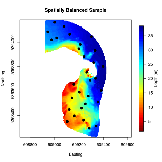
Figure 2.2: A uniform inclusion probability sample for Governor Island
Preference shallow environments
The equal inclusion probability design (Figure 2.2) assumes that all sites are equally advantageous to sample. Previously, we mentioned that this may not be an efficient approach to sampling. In particular, it can be advantageous to over-sample sites/regions that have greater variability. In the Governor Island reserve, this corresponds to the shallower depths as these typically are more heterogeneous and biodiverse on the east coast of Tasmania. We can design a survey with this in mind by increasing the probability that shallow sites will be sampled (i.e. by increasing their inclusion probabilities). This has the obvious effect of also decreasing the probability that deeper sites will be sampled (Figure 2.3). The code below shows how this can be done. It is a little more involved, but most of the complexity comes from detail. The approach is simple though: 1) find the empirical distribution of depths in the reserve; 2) define the inclusion probabilities based on this empirical distribution; and 3) sample according to those inclusion probabilities. We will sample a few more sites (n = 100), just to make the effect of the depth adjustment clear.
###########################################################################
####    Spatially balanced design -- Depth biased inclusion probs     ####
####    Foster et al. NESP Biodiversity Hub Field Manuals              ####
###########################################################################

**par**( mfrow=**c**(1,3), mar=**rep**( 4, 4))
n <- 100
#The number of 'depth bins' to spread sampling effort over.
nbins <- 4
#force the breaks so R doesn't use 'pretty'
breaks <- **seq**( from=**min**( bth.orig.grid$Depth, na.rm=TRUE),
    to=**max**( bth.orig.grid$Depth, na.rm=TRUE), length=nbins+1)
#Find sensible depth bins using pre-packaged code
tmpHist <- **hist**( bth.orig.grid$Depth, breaks=breaks, plot=FALSE)
#Find the inclusion probability for each 'stratum'
tmpHist$inclProbs <- (n/(nbins)) / tmpHist$counts
#Matching up locations to probabilties
tmpHist$ID <- **findInterval**( bth.orig.grid$Depth, tmpHist$breaks)
#A container for the design
design <- **data.frame**( siteID=1:**nrow**( bth.orig.grid),
    Easting=bth.orig.grid$Easting, Northing=bth.orig.grid$Northing,
    Depth=bth.orig.grid$Depth, inclProb=tmpHist$inclProbs[tmpHist$ID])
#Plot the depths and the inclusion probabilties
**with**( design, **plot**( Depth, inclProb, main="Inclusion Probabilities",
    ylab="Inclusion Probabilities", xlab="Depth (m)", pch=20, cex=1.4))
#Plot the inclusion probabilities in space
**with**( design,
    **image.plot**( uniqueEast, uniqueNorth,
        **matrix**( inclProb, nrow=**length**( uniqueEast), byrow=FALSE),
        xlab="", ylab="", main="Inclusion Probability", asp=1,
        ylim=NLims, xlim=ELims))
#Take the Sample using the inclusion probabilities
samp <- **quasiSamp**( n=n, dimension=2,
    potential.sites = design[,**c**("Easting","Northing")],
    inclusion.probs=design$inclProb, nSampsToConsider=100*n)
#Plot the design
**with**( design, **image.plot**( uniqueEast, uniqueNorth, DepthMat,
    xlab="", ylab="", main="Spatially-Balanced Sample", asp=1,
    ylim=NLims, xlim=ELims,


    col=rev(tim.colors())))
points( samp[,c("Easting","Northing")], pch=20, cex=2)
write.csv( design, file="design.csv", row.names=FALSE)
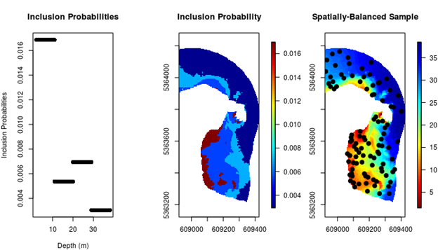
Figure 2.3: (Left panel) The empirical distribution of the 4 different depth bins. (Middle panel) The spatial distribution of the depth bins. (Right panel) A non-uniform spatially balanced sample, with inclusion probabilities based on the distribution of depths throughout the region. Shallow sites have been over-represented in the sample.
Incorporate legacy sites
Here, for edification purposes, we provide an illustration of how to design a spatially-balanced survey that accounts for the locations of legacy sites, which are those sites that we wish to include in the survey. The most likely reason for including legacy sites is that they have been sampled before as part of a previous randomisation process. Various names exist for legacy sites, including ‘reference sites’, and perhaps even ‘sentinel sites’ in some situations.
In our example, we first generate legacy sites and then generate more sites around them. To provide a little extra spice to the design we try to mimic the learning process: the n = 6 legacy sites are chosen with uniform probabilities (as we would do when there is no information about the area) and then the n = 15 new sites are chosen with a depth gradient altering the inclusion probabilities (Figure 2.4). This example therefore incorporates elements of the previous two examples.
###########################################################################
####    Spatially balanced design -- Legacy Sites (biassed incl probs) ####
####    Foster et al. NESP Biodiversity Hub Field Manuals              ####
###########################################################################

#set up the plotting structure
par( mfrow=c(2,2), mar=c(3,3,3,3))
#number of samples
n_l <- 6
##Take the sample for the legacy sites.
#Here they are a spatially balanced sample but in practice
# they would be supplied from a previous randomisation process
samp_legacy <- quasiSamp( n=n_l, dimension=2,
    potential.sites = bth.orig.grid[,c("Easting","Northing")],
    inclusion.probs=!is.na( bth.orig.grid$Depth))
#plot the legacy sites
with( bth.orig.grid, image.plot( uniqueEast, uniqueNorth, DepthMat,
    xlab="Easting", ylab="Northing", main="Legacy Sites",
    legend.lab="Depth (m)", asp=1, ylim=NLims, xlim=ELims,
    col=rev(tim.colors()), legend.mar=8.1))
points( samp_legacy[,c("Easting","Northing")], pch=17, cex=2)
#plot the depth-based inclusion probabilities
# scale first to sum to n=15
n <- 15
design$inclProb <- n * design$inclProb / sum( design$inclProb, na.rm=TRUE)
with( design,
    image.plot( uniqueEast, uniqueNorth,
        matrix( inclProb, nrow=length( uniqueEast)),
        xlab="", ylab="", main="Inclusion Probability", asp=1,
        ylim=NLims, xlim=ELims, legend.mar=8.1))
##Depth-based inclusion probabilities
#Alter the inclusion probabilities for the next sample
# inclusion probs taken from previous example
p2 <- alterInclProbs( legacy.sites=as.matrix(
    samp_legacy[,c("Easting","Northing")]),
    potential.sites=bth.orig.grid[,c("Easting","Northing")],
    inclusion.probs=design$inclProb)
#plot the altered inclusion probabilities
with( design,
    image.plot( uniqueEast, uniqueNorth,
      matrix( p2, nrow=length( uniqueEast)), ylim=NLims, xlim=ELims,
      xlab="", ylab="", main="Altered Inclusion Probability", asp=1, legend.mar=8.1))
##Take the new sample, spatially balanced around the legacy sites
samp <- quasiSamp( n=n, dimension=2,
    potential.sites = design[,c("Easting","Northing")],
    inclusion.probs=p2, nSampsToConsider=100*n)
#plot legacy sites and new sample sites.
with( design, plot( Easting, Northing,
    col=c('white',grey(0.9))[1+!is.na(inclProb)], ylim=NLims, xlim=ELims,
    xlab="", ylab="", main="Combined Sample Locations", asp=1))
points( samp_legacy[,c("Easting","Northing")], pch=17, cex=2, col='red')
points( samp[,c("Easting","Northing")], pch=20, cex=2)
legend( "bottomleft", c("Legacy Sites", "New Sites"), pch=c(17,20), pt.cex=2,
    col=c('red','black'), bty='n')
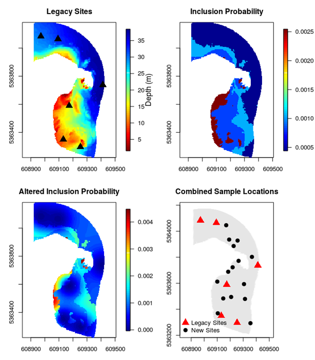
Figure 2.4: A spatially balanced design for Governor Island that incorporates legacy sites and has depth-varying inclusion probabilities (shallow sites are over-represented).
Case study summary
We have now seen how to generate three different kinds of designs: 1) a spatially balanced design with equal inclusion probabilities for when little is known about the sources of variation of the system; 2) a spatially balanced design with unequal inclusion probabilities for when we think we know where the locations with higher variance are likely to be; and 3) a spatially balanced design for when we have legacy sites that we want to take a repeat sample.
If future researchers wish to re-survey the area at some point in the future, then they have a choice to make: (i) Do they wish to revisit the same sites (to get a good temporal estimate)? (ii) Do they choose a new set of sites (to get a good spatial estimate)? Or (iii) Do they assume that the temporal change is not important and include the previous survey as part of the sample? This last scenario would be performed efficiently by using the original sample locations as legacy sites and spatially balance the new sample locations around those (as was done in the example). It will usually be sensible to combine these objectives by repeating some (not all) of the samples but choosing some new locations as well.